Tinkering with gradient boosting

TL;DR

We look at two approaches to tailor gradient boosting with a custom loss function: analytic derivation of the gradient and automatic differentiation via autograd. Code is available in a Jupyter notebook.

When procrastination gets the better of me, I sometimes find myself wandering about the Elysian fields of lost time better known as YouTube. On rare occasions I end up stumbling on something useful, like this talk by Trevor Hastie given at an H2O World event, a walkthrough of bagging and boosting. Much like the accompanying book, it’s peppered with tidbits of indispensable practical advice. One comment in particular caught my ear:

These models [random forests and gradient boosting] are really very open to tinkering.

This innocuous statement is interesting because it stands in stark contrast to the way tree ensembles are typically thought of, as off-the-shelf black box algorithms controlled by a few knobs, such as tree depth, number of trees, etc. In fact, in Elements of Statistical Learning gradient boosting is explicitly marketed as an off-the-shelf solution:

A gradient boosted model (GBM) is a generalization of tree boosting that attempts to mitigate these problems, so as to produce an accurate and effective off-the-shelf procedure for data mining.

Gradient boosting

What is it about gradient boosting that make it amenable to tinkering? Let’s revisit. For a given response vector \(y\), gradient boosting seeks to minimize the loss \(L(y, f(x))\) by fitting an additive model \[ f(x) = \sum_{k} \beta_k h_k(x) , \] with \(h_k(x)\) the base learners, typically trees. The algorithm follows a forward stagewise structure, which is stats-speak for a greedy approach that iteratively adds new learners to the model without going back and changing the parameters and coefficients of learners that were previously added, i.e.,

The \(h_k\)’s are found by fitting a base learner to the negative gradient of the loss evaluated at the current model estimate

In other words, in each iteration we compute \(-r_k\) and then use it as a response for fitting the base learner \(h_k\) (Friedman calls these \(r_k\)’s “pseudo-responses”).

Reviewing the gradient boosting procedure, we see that (a) by construction, it is defined for an arbitrary loss function, so in principle we can use it to optimize any loss function we can conjure, and (b) the forward stagewise structure means that at iteration \(k\) we don’t need to know anything about the stuff that’s in \(f_{k-1}(x)\), which opens up possibilities for creating various hybrids. This post will focus on (a), hopefully we’ll get to (b) in a later post.

Custom loss with analytical gradients

We will use xgboost for tinkering purposes. Beyond the fact that it’s lightning fast, its python API is well designed and quite flexible, and as we’ll see it’s dead simple to plug in an arbitrary loss function. The underlying model is not 100% faithful to Friedman’s gradient boosting as popularized in R’s gbm or in scikit-learn. One notable difference is that it uses second-order information about the loss function for minimization (a diagonal approximation of the Hessian).

Running xgboost with an arbitrary loss function is as easy as writing a function that spits out the gradient of the loss evaluated at the current prediction. As a simple example, suppose our loss function is the popular squared loss

Its gradient w.r.t. \(f\) is

That was easy! For more complex expressions, having a matrix calculus cheat sheet around is handy. Now we just have to implement this gradient as a python function. Oh wait, we said something about the Hessian earlier, no? We’ll follow sage advice from the author of xgboost about specifying second-order information and use a constant for the diagnoal of the Hessian (for squared loss the diagonal of the Hessian is a constant anyway, but for other loss functions it can be tricky to calculate). Here is the implementation of \(L_2\) loss, \(L_1\) loss, and Huber loss (What? These are already implemented out of the box in scikit-learn?? But… well… oh bother).

def l2loss(preds, dtrain):
    labels = dtrain.get_label()
    grad = preds - labels
    hess = np.ones_like(grad)
    return grad, hess

def l1loss(preds, dtrain):
    labels = dtrain.get_label()
    grad = np.sign(preds - labels)
    hess = np.ones_like(grad)
    return grad, hess

def huberloss(alpha=90):
    def loss(preds, dtrain):
        labels = dtrain.get_label()
        diff = preds - labels
        delta = np.percentile(np.abs(diff), alpha)
        grad = diff
        grad[np.abs(diff) > delta] = delta*np.sign(diff[np.abs(diff) > delta])
        hess = np.ones_like(grad)
        return grad, hess
    return loss

To test our newly acquired loss functions, we’ll use the California housing dataset, randomly split into 80%/20% training/test samples. As Hastie et al. point out, \(L_1\) or Huber are robust alternatives to \(L_2\) loss that may be useful when the data is riddled with outliers. So it’d be interesting to see whether we gain anything from using robust loss functions in place of squared loss. We’ll train xgboost with each of the 3 loss functions above and compare.

# xgboost configuration
n_estimators = 1000
xgb_params = {'max_depth' : 3, 'eta' : 0.05, 'seed' : 12345, 'silent' : 1}
# Train models
models = [xgb.train(xgb_params, dtrain, n_estimators, obj=o) for o in (l2loss, l1loss, huberloss(90))]

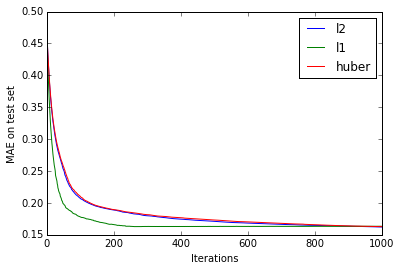
This is what the (mean absolute) error on the test set looks like as the number of trees varies:

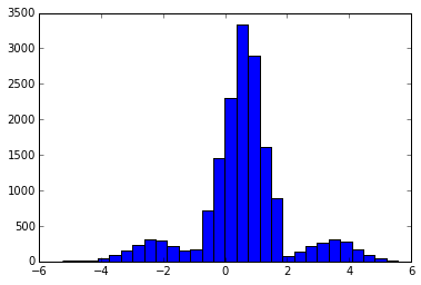
Disappointingly, after a sufficient number of iterations, there are no apparent accuracy gains from using the robust loss functions, though \(L_1\) loss does reach lower error rates faster than the other two loss functions. But we won’t give up that quickly - let’s see what happens when we add more outliers. We’ll use a simple bimodal distribution with two Gaussian peaks to simulate outliers in the response variable:

def add_outliers(y, frac=0.01, dist=5.0):
    sd = np.std(y)
    ind = np.random.choice(len(y), frac*len(y), replace=False)
    yo = y.copy()
    yo[ind] = yo[ind] + np.sign(np.random.normal(size=len(ind))) * \
    		  np.random.normal(loc=dist*sd, scale=sd, size=len(ind))
    return yo

Here’s the distribution of the corrupted response values with 20% outliers:

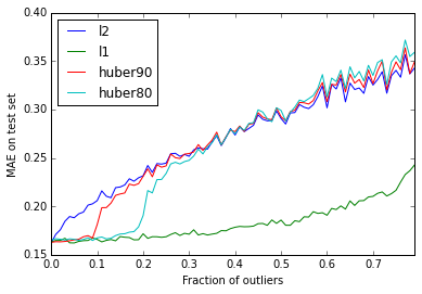
Now that we have a way to corrupt the data, we’ll run a Monte Carlo simulation, varying the fraction of outliers in the response, and see how the performance of the algorithm degrades with different loss criteria.

fracs = np.arange(0.0, 0.8, 0.01)
mae = []
for frac in fracs:
    # Add outliers to training data
    dtrain_corrupt = xgb.DMatrix(
    	X_train,
    	add_outliers(y_train, frac=frac, dist=5.0),
    	feature_names=feature_names)
    # Train models
    models = [xgb.train(xgb_params, dtrain_corrupt, n_estimators, obj=o) \
    	for o in (l2loss, l1loss, huberloss(90), huberloss(80))]
    # Compute validation errors    
    mae.append([mean_absolute_error(y_test, m.predict(dtest)) for m in models])

Two interesting findings jump out. First, \(L_1\) loss proves exceptionally resilient to outliers, with noticeable degradation in accuracy only for 50% or more corrupt observations. Second, models trained with Huber loss act as a hybrid, switching from \(L_1\)-like behavior to \(L_2\)-like behavior when the fraction of outliers exceeds the Huber outlier percentile.

Fun with autograd

What if the loss function we want to minimize is particularly hairy and the thought of deriving its gradient analytically is enough to steer us clear of this whole mess? Well, a convenient by-product of the ongoing deep learning revolution is the abundance of libraries for doing automatic differentiation. For python, the best known library is Theano, which is great for defining and training deep nets, but is overkill for our purposes. Instead, we’ll use autograd, a library for automatic differentiation of python and numpy code with a beautifully minimalistic API. Here’s how to modify the code above to define our own \(L_2\) loss and compute its gradient with autograd.

import autograd.numpy as np
from autograd import grad

def l2_obj(x):
    return 0.5 * np.sum(x ** 2)

def l2autograd(preds, dtrain):
    labels = dtrain.get_label()
    grad_l2obj = grad(l2_obj)
    g = grad_l2obj(preds - labels)
    h = np.ones_like(g)
    return g, h

From a line count perspective, not so impressive: we had 5 lines of code, now we have 8. The gain comes from readability and ease of prototyping: we define the loss function explicitly (rather than its gradient), and we can easily test variations without having to recalculate the gradient each time. The only interaction with autograd is the call to grad(), supplying the loss function as an argument. Pretty sweet! It also handles a pretty wide array of numpy primitives without complaining; here’s an implementation of Huber loss, same idea.

def huberobj(delta):
    def obj(x):
        return 0.5*np.sum(np.where(np.abs(x) <= delta, (x) ** 2, 2*delta*np.abs(x) - delta**2))
    return obj

def huberautograd(alpha=90):
    def loss(preds, dtrain):
        labels = dtrain.get_label()
        e = preds - labels
        delta = np.percentile(np.abs(e), alpha)
        obj = huberobj(delta)
        obj_autograd = grad(obj)
        g = obj_autograd(e)
        # Handle nan's in the gradient
        g[np.isnan(g)] = 0
        h = np.ones_like(g)
        return g, h
    return loss

For fun, we can check that the two approaches, analytical gradients and autograd, give the same results.

# Train models using l2 loss
models = [xgb.train(xgb_params, dtrain, n_estimators, obj=o) for o in (l2loss, l2autograd)]
# Test that we get the same thing
preds = [m.predict(dtest) for m in models]
print(mean_absolute_error(preds[0], preds[1]))
# > 0.0

Performance benchmark

We looked at two ways to train gradient boosting with a custom loss function, and we are ready to tackle the world’s machine learning problems again. Of course, nothing in life is free, so it will come as no surprise that the ability to conveniently specify an arbitrary loss function in python while still using xgboost’s C++ implementation comes at a cost. How much? let’s take a look. We’ll compare 3 approaches to gradient boosting regression with squared loss: the native xgboost implementation (C++), an implementation using the analytical form of the gradient, and an implementation using autograd.

n_estimators = 1000
xgb_params = {'max_depth' : 6, 'eta' : 0.05, 'seed' : 12345, 'silent' : 1}

%timeit xgb.train(xgb_params, dtrain, n_estimators)
> 1 loops, best of 3: 4.12 s per loop

%timeit xgb.train(xgb_params, dtrain, n_estimators, obj=l2loss)
> 1 loops, best of 3: 13.3 s per loop

%timeit xgb.train(xgb_params, dtrain, n_estimators, obj=l2autograd)
> 1 loops, best of 3: 13.8 s per loop

At first glance, the cost seems prohibitive, with the custom implementations more than 3x slower than the native implementation. But on second thought, this is probably a very pessimistic estimate; for realistically-sized problems, xgboost spends the majority of the time building trees and a small chunk of time evaluating the gradient, so the performance hit would be much smaller.